
More Information
Submitted: February 25, 2021 | Approved: March 15, 2021 | Published: March 16, 2021
How to cite this article: Swan BQ. Economic disparities and suicides: The dynamic panel data analyses of 50 states in the United States. J Forensic Sci Res. 2021; 5: 020-029.
DOI: 10.29328/journal.jfsr.1001023
ORCiD ID: orcid.org/0000-0001-9822-7550
Copyright License: © 2021 Swan BQ, et al. This is an open access article distributed under the Creative Commons Attribution License, which permits unrestricted use, distribution, and reproduction in any medium, provided the original work is properly cited.
Keywords: Dynamic panel data; Suicide; Economic inequality; Arellano-Bond estimate; Gini index

Economic disparities and suicides: The dynamic panel data analyses of 50 states in the United States
Bruce Q Swan*
State University of New York, Buffalo State, USA
*Address for Correspondence: Bruce Q Swan, Ph.D., State University of New York, Buffalo State, USA, Tel: (716) 878-6429; Email: [email protected]
The economic inequalities associated with suicide risks among 50 states in the United States were identified in this paper to form the dynamic panel data set from 1981 to 2016. The effects of growing income inequalities on suicides in the Unites States were estimated using the Arellano–Bond method. This paper is the first to associate the social inequalities with suicides using the state-level dynamic panel data in America. It is found that the change of unemployment rates significantly and positively impact the changes of the overall suicides rates, female and male suicides rates. The changes of Top 10% income index are uniformly positive to the change of female, male and overall state-level suicide rates. The Gini index has positive correspondence within the overall and female groups, along with the insignificantly vague evidence within the male groups. The potential endogeneity problem inferring from the fixed effect estimation has been also investigated accordingly.
JEL Classification: A13, A14, I18.
Suicide has been one of the top leading causes of death in the United States. The number of suicides per 100,000 Americans rose 30.4% (2015) from 1999 to 2015. However, suicide rates in other developed nations like Western European nations have generally fallen in the same period of time. According to the World Health Organization [1], suicide rates fell in 12 of 13 Western European nations between 2000 and 2012.
It is also noted that the income inequality has increased consistently in the U.S. during the past decades, perhaps more than at any time in the history. On the contrary, this phenomena did not exist in western European countries. It is reported by the U.S. Census Bureau [2] and the World Wealth Report, that the assets of top 5% in the U.S. increase significantly even during the recessions while the high-salary and mid-class jobs have been decreased especially after the financial crisis in 2008. Based on Internal Revenue Service reports, in 1980 the richest 1% of Americans took 1 of every 15 national income dollars, whereas now they take 3 of every 15 national income dollars. This implies that the richest 1% has tripled their cut of America’s income shares just in one generation. In general, according to the report from World Bank [3], the United States was concluded to be the most economically stratified society in the developed nations.
In the reports of health disparities and inequalities in the United States and from Centers for Disease Control and Prevention (CDC) [4,5], the socio-economic position may have significant effects on health and mortality including suicides. Some previous research had also generally found that the higher the level of income inequality in the urban areas of the United States, the higher the probability of death by suicide would be. The socio-economic conditions of the places where persons live and work may have an even more substantial influence on health. According to social strain theory by Sun & Zhang, [6] when there’s a large gap between different income levels, those at or near the bottom struggle more, making them more susceptible to addiction, criminality and mental illness than those at the higher level.
However, it has been long term noted that the work on suicide’s relationship to income and social inequality is still scant in the United States. The effects of growing social and income inequalities on suicides in the U.S. during the last three decades are new, confusing and even contradictive. The rigorous researches are needed to update what have been known about the present American context. In this paper, the socio-economic indicators and the suitable statistical models and methods will be applied to test the effects of suicide risk of socio-economic inequalities. I hypothesize that the economic disparities in the U.S. play significant roles on the suicides, the groups of different sex or ages have different responses to these risk factors, and the strength of the responses will also be distinct.
Antonio Andrés [7] did an investigation of the relation among income inequality, unemployment, and suicides using a panel data of 15 European countries. They found that suicide rates in these countries were not sensitive to income levels, female labor participation rates and unemployment. Although income levels can give some descriptions to people’s economic situations, they didn’t have enough power to explain suicides as shown in the above work. Using a panel of the United States from 1996 to 2005 with monthly aggregate data on suicides, Classen & Dunn [8] found the different measures of unemployment exhibit different explanatory power for suicide risk, and some measures have adverse effects on suicide rates. Many researchers have indicated that different social inequalities, especially income inequality impacts a lot on multiple levels of societies, correlating with, if not causing directly, less happiness, poorer mental and physical health leading to deaths, mainly suicides. Therefore, in this paper, I will select income inequality instead of income levels.
Andres and Halicioglu [9] examined the determinants of suicides in Denmark from1970 to 2006 and found that suicide was associated with a range of macro socio-economic factors but the strength of the association can differ by gender. Julie Phillips, [10] found relations of factors with temporal and spatial patterns to suicide rates across American States. She use pooled cross-sectional time-series data for the 50 states over the 25-year period to examines how well demographic, economic, social, and cultural factors, are associated with the 1976–2000 patterns in overall suicide rates and suicide by firearms and other means.
Hintikka and Pirjo [11] did a study on associations between suicide mortality, unemployment, divorce rate and mean alcohol consumption in Finland from 1985 to 1995. They reported that the association between suicide and unemployment or divorce rates was not found. Nancy & Katherine, [12] did a research on socioeconomic disparities in health. They claimed that, socioeconomic status (SES) underlies health behaviors and chronic stress associated with lower SES may increase morbidity and mortality. To reduce SES disparities in population health will require government policy initiatives addressing the components of socioeconomic status (income, education, and occupation) as well as the pathways by which these affect health. Besides the above work, Adler and Rehkopf [13] showed that although health was consistently worse for individuals with few resources and for blacks as compared with whites, the extent of health disparities varies by outcome, time, and geographic location within the United States. There should be more evidences to support the associations between the factors of health disparities and suicides.
Ceccherini [14] utilized unit root and co-integration tests to test the associations over time between economic factors and suicide rates in four countries. Different to theirs, we will use the dynamic panel dataset to do the estimations. Among some other related works, Yang, Stack and Lester [15,16] found that both the unemployment rate and the female participation rate are powerful predictors of the suicide rates. Swan, Sun, et al. [17] look at the taxation effect on cross-state smuggling using rational addiction models. They show how the taxation effect can be a valid instrumental variable for lagged and future consumption together with the local price series using dynamic panel data estimations.
About the indices of economic inequality, I use the dataset derived by Frank, [18]. Before Frank’s dataset, most indicators were primarily from the two prior income inequality data sets: the international panel of Deininger and Squire, and the U.S time-series data of Piketty and Saez. Deininger and Squire offer inequality measures for a wide panel of nations with several time-series observations for each nation beginning in the year 1960. Piketty and Saez, on the other hand, constructed a high-frequency U.S. time-series data set. Unlike the large-N and small-T panel of Deininger and Squire, the Piketty and Saez datasets contain up to 85 annual observations for the U.S. covering the period 1913-1998.
Different from the previous datasets, Frank’s new panel applied the IRS income tax filing data together with the BEA (the Bureau of Economic Analysis) calculation of per capita state income, to construct a comprehensive state-level panel of annual income inequality measures. The innovated dataset can reveal the significant state-level variations, both timely and regionally.
Data
The state-level suicide rates are downloaded from CDC’s WISQARS (Web-based Injury Statistics Query and Reporting System), an interactive and online database that provides fatal and nonfatal injury and suicide data from a variety of trusted sources. In the CDC mortality report and report from Agency for Healthcare Research and Quality (AHRQ) [19], it stated that suicide has been a leading cause of death in the US, and suicide rates increased nearly every state from 2000 through 2016. In this period, the whole national suicide rates went up more than 30% in half of states, from 10.4 to 13.5 per 100,000 population, increasing on average by about 1% per year from 2000 through 2006 and by 2% per year from 2006 through 2016. For males, the rate increased 21%, from 17.7 in 2000 to 21.4 in 2016, and for females, the rate increased 50%, from 4.0 in 2000 to 6.0 in 2016. In 2016, suicide became the second leading cause of death for population group with ages 10–34 and the fourth leading cause for ages 35–54. Although the Healthy People 2020 target is to reduce suicide rates to 10.2 per 100,000 by 2020, the whole national suicide rates have still steadily increased in recent years. In figure 1, we can see that the national suicide rates increased consistently from 2010 to 2016, and in table1, about 2/3 of all the states reach the maximum suicides rates in the most recent years.
About the socio-economic indicators, the state-level unemployment rates, GINI index and the top 10% income ratio in the United States will be applied in this investigation. Frank, [18] published the lists of state level panel of annual inequality measures, in which the IRS income tax filing data together with the BEA (the Bureau of Economic Analysis) calculation of per capita state income have been applied to construct a comprehensive state-level panel of annual income inequality measures. Although IRS income data has several important limitations, including the censoring of individuals below a threshold level of income and the discrepancy in tax units, Frank’s panel made innovations on covering an under-exploited unit of observation, American states, and that is large in both cross-sections and time-series observations. While a panel of American states is more homogenous than most cross-national panels, it retains a useful degree of heterogeneity derived from each state’s unique political/institutional history, and regional heritage.
In this paper, GINI index and Top 10% income ratio from Frank’s datasets are selected, with the data entry in the last year 2016 interpolated from the historical data. Gini index, or Gini ratio is a measure of statistical dispersion designed to represent the income distribution of a nation’s residents, and is the most commonly used measurement of economic and social inequality. The top 10% income ratio measures the percentage of the income from the 10% families covering the whole income. The larger GINI index and the Top 10% income ratio are, the income distribution in a nation is more unequally distributed, i.e. the more unequal. The state unemployment rates 1981-2016 were seasonally adjusted and downloaded from Federal Reserve Bank of St. Louis (FRED) (Table 1), https://fred.stlouisfed.org/
| Table 1: The summary of the suicides in each state of the U.S 1981-2016. | |||||
| The United States | Average rate | Standard Deviation | minimum year | maximum year | Autoregressive coefficient |
| Whole USA | 11.92 | 0.81 | 2000 | 2016 | 0.95 |
| Alabama | 12.63 | 1.17 | 1981 | 2016 | 0.73 |
| Alaska | 18.62 | 4.50 | 1988 | 2015 | 0.60 |
| Arizona | 17.27 | 1.29 | 2001 | 1987 | 0.78 |
| Arkansas | 14.02 | 1.88 | 1989 | 2015 | 0.82 |
| California | 11.65 | 2.14 | 2001 | 1982 | 0.97 |
| Colorado | 17.34 | 1.52 | 1999 | 2016 | 0.63 |
| Connecticut | 8.71 | 0.81 | 2007 | 2016 | 0.61 |
| Delaware | 11.78 | 1.47 | 1998 | 1987 | 0.50 |
| District of Columbia | 6.32 | 1.65 | 2000 | 1982 | 0.30 |
| Florida | 14.21 | 1.15 | 1999 | 1982 | 0.86 |
| Georgia | 12.16 | 1.14 | 2006 | 1991 | 0.80 |
| Hawaii | 10.73 | 1.61 | 2005 | 2010 | 0.53 |
| Idaho | 17.48 | 1.98 | 2000 | 2015 | 0.58 |
| Illinois | 9.51 | 1.03 | 1997 | 1985 | 0.85 |
| Indiana | 12.52 | 1.03 | 1999 | 2016 | 0.78 |
| Iowa | 11.79 | 1.26 | 2000 | 2016 | 0.60 |
| Kansas | 13.11 | 1.63 | 2001 | 2016 | 0.68 |
| Kentucky | 13.84 | 1.31 | 1999 | 2015 | 0.75 |
| Louisiana | 12.67 | 1.29 | 2003 | 1986 | 0.78 |
| Maine | 13.49 | 1.64 | 2003 | 2013 | 0.36 |
| Maryland | 9.65 | 0.98 | 1999 | 1986 | 0.76 |
| Massachusetts | 7.92 | 0.87 | 2000 | 1987 | 0.78 |
| Michigan | 11.65 | 1.04 | 2000 | 2015 | 0.84 |
| Minnesota | 11.13 | 1.14 | 2000 | 2015 | 0.83 |
| Mississippi | 12.16 | 1.04 | 1982 | 2012 | 0.65 |
| Missouri | 13.64 | 1.45 | 2003 | 2016 | 0.82 |
| Montana | 20.26 | 2.33 | 1982 | 2016 | 0.69 |
| Nebraska | 11.28 | 1.19 | 2009 | 1986 | 0.32 |
| Nevada | 21.85 | 3.05 | 2007 | 1982 | 0.71 |
| New Hampshire | 12.74 | 1.78 | 2004 | 2014 | 0.50 |
| New Jersey | 7.09 | 0.60 | 2005 | 2014 | 0.60 |
| New Mexico | 19.58 | 1.60 | 1998 | 1988 | 0.59 |
| New York | 7.33 | 0.82 | 2000 | 1981 | 0.74 |
| North Carolina | 12.31 | 0.75 | 1998 | 1990 | 0.62 |
| North Dakota | 12.93 | 2.35 | 1981 | 2016 | 0.78 |
| Ohio | 11.28 | 1.24 | 2003 | 2016 | 0.74 |
| Oklahoma | 15.20 | 1.95 | 1990 | 2016 | 0.88 |
| Oregon | 15.91 | 1.12 | 1999 | 2014 | 0.56 |
| Pennsylvania | 11.67 | 0.99 | 2001 | 2016 | 0.86 |
| Rhode Island | 9.29 | 1.66 | 2005 | 1987 | 0.55 |
| South Carolina | 12.37 | 1.30 | 1988 | 2016 | 0.62 |
| South Dakota | 14.85 | 2.32 | 1992 | 2015 | 0.52 |
| Tennessee | 13.56 | 1.00 | 2001 | 2016 | 0.78 |
| Texas | 12.17 | 1.27 | 1999 | 1986 | 0.92 |
| Utah | 16.84 | 2.20 | 1999 | 2015 | 0.81 |
| Vermont | 14.48 | 2.22 | 1994 | 2014 | 0.40 |
| Virginia | 12.29 | 1.01 | 2000 | 1982 | 0.82 |
| Washington | 13.86 | 1.01 | 2001 | 1986 | 0.61 |
| West Virginia | 14.19 | 1.81 | 1988 | 2016 | 0.78 |
| Wisconsin | 12.41 | 1.02 | 1997 | 2016 | 0.72 |
| Wyoming | 20.67 | 2.63 | 2001 | 2015 | 0.43 |
The dynamic panel data model and Arellano-Bond estimate will be applied to do the data analyses. It was firstly verified that the suicide rates in the U.S has significant autocorrelations, then the relation between the dependent variable, Sit, the suicide rates in the U.S, and the covariates Xit, can be modeled by the dynamic specification:
(1)
and,
(2)
where Xit is the vector of covariates, ηi denotes the unobserved individual-specific and time-invariant hetero-geneity, εit is the idiosyncratic error terms.
The dynamic panel data model in the above permits the distinction between the long term relationship and the short-run dynamics. In the model, Xit is a vector containing both contemporaneous and lagged values of explanatory variables. The above specification has several important specifications, i.e. static models, distributed lag and differenced specifications. When the strict exogeneity assumption is violated, those commonly used static panel data techniques such as fixed effect estimators are inconsistent, because these estimators require strict exogeneity. Therefore the conventional fixed and random effects models will produce biased coefficients. Some more effective methods have been developed to avoid such problems. The Arellano–Bond method [20] is one of them and used in this paper. Using this method, the first difference of the regression equation are taken to eliminate the fixed effects. Then, deeper lags of the dependent variable are tested as instruments for the differenced lags of the dependent variable could be endogenous. On the other hand, in those traditional panel data methods, adding deeper lags of the regressors reduces the number of observations available. Then it creates a trade-off: adding more lags provides more instruments, but reduces the sample size. In general, the linear dynamic panel data models contain a few lags of the dependent variable as covariates and unobserved panel level effects, fixed or random.
The Arellano–Bond method effectively circumvents this problem. Arrelano and Bond firstly solved these problems, using earlier lagged values of x and y as the instrumental variables and a generalized method of moments (GMM) estimator (1991). Later on, more computational methods have been developed to do the estimations for Arrelano Bond tests. By construction, the unobserved panel level effects are correlated with the lagged dependent variables, making standard estimators inconsistent. In his paper, Arrelano Bond tests are used to estimate the parameters. The packages and tools used in the paper are STATA SE14 and MATLAB2015. The command xtabond [21] implements the estimator. It requires that there would be no autocorrelations in the idiosyncratic errors. For a related estimator that uses additional moment conditions, but still requires no autocorrelation in the idiosyncratic errors.
The estimation results are summarized as follows in tables 2,3. The first part in table 2 shows the coefficients of suicide rates cross states overall and individual female and male suicide rates with income inequality status or independent variables, unemployment rate, top 10% income index, and Gini index respectively, and all show significantly positive relationship without fixed effects. In different specifications, lagged values of suicide rates are all significant for 5% level. All the coefficients of lagged suicide rates are significant for both 5% level and 1% level. The positive and consistent coefficient estimates of Xi,t-1 confirm that the current year’s measurable increment for suicide rate is adaptive to lagged-one-year’s values. Moreover, the insignificant coefficient estimates of Xi,t-2 reject the lagged-two-year’s dependence, which supports the model in table 2. In our framework, the relationship we examined for series Xi,t-1 are statistically significant in most cases.
| Table 2: The Arellano-Bond Results by Using “Suicide Rate” as Dependent Variable. |
| This table is set for the results from the model according to the equation (2) in model framework, applying Arellano-Bond methods for cross-sectional time series make the estimation for the causality of the employment level and the national income status, here, unemployment rate, top ten percent income index, Gini index, on the suiside rate. The first column contains the independent variables we examined. Intercepts are expressed later. All the entries are the values of estimators correspond to the independent variable in each row. Results here for comparison are GMM estimates. On the other hand, Arellano-Bond test that average autocovariance in residuals of order 1 is almost 0 not failed in 5% level for all alternative specifications, and failed in 5% level in residuals of order 2 for all alternative specifications. Wald test statistics ranges from 2475.05 to 10565.59, which shows the efficiency of the alternative models. The GMM overidentification Sargan test shows the two-step GMM estimators which are mostly statistically insignificant at the 5% level. “*” represents the 5% significance, “**” represents the 1% significance. The paraphrased figures are the standard deviations, and the bracketed ones are the p–values. |
| Overall Suicide Rates t-value Female suicide rates t-value Male suicide rates t-value |
| Sui Lag 1 0.6178*** 92.71 0.5210*** 32.97 0.4490*** 30.20 |
| [0.6048 0.6309] 0.0000 [0.4900 0.5520] 0.0000 [0.4198 0.4781] 0.0000 |
| Unemp Rates 0.0976*** 30.17 0.0878*** 34.55 0.1305*** 30.82 |
| [0.0905 0.1046] 0.0000 [0.0828 0.0928] 0.0000 [0.1222 0.1388] 0.0000 |
| Top10 Index 0.0408*** 20.34 0.0478*** 14.40 0.0539*** 9.40 |
| [0.0375 0.0443] 0.0000 [0.0413 0.0543] 0.0000 [0.0427 0.0652] 0.0000 |
| Gini Index 1.9539*** 10.23 2.8222*** 13.64 -2.5467** -2.25 |
| [1.5793 2.3285] 0.0000 [2.4166 3.2277] 0.0000 [-3.7132 -1.3802] 0.0250 |
| Constant Term 2.6638*** 13.22 1.3470*** 3.67 11.1968*** 27.73 |
| [2.2687 3.0589] 0.0000 [0.9509 1.7431] 0.0000 [10.4053 11.9882] 0.0000 |
| Wald chi2(3) 10565.59 7595.50 2475.05 |
| p < 0.0000 p < 0.0000 p < 0.0000 |
| Sargan test 47.6928 46.0360 49.1542 |
| p > 1.0000 p > 1.0000 p > 1.0000 |
| AB AR(1) -3.4933 -4.7841 -3.7840 |
| [0.0005] [0.0000] [0.0002] |
| AB AR(2) 1.7917 1.1597 1.6161 |
| [0.0732] [0.2462] [0.1061] |
| For comparing, this following table is set for the results from the model according to the equation (2) in model framework, applying fixed effect methods for cross-sectional time series make the estimation for the causality of the employment level and the national income status, here, unemployment rate, top ten percent income index, Gini index, on the suicide rate. The first column contains the independent variables we examined. Intercepts are expressed later. All the entries are the values of estimators correspond to the independent variable in each row. Results here for comparison are 2SLS estimates. On the other hand, F test statistics ranges from 162.07 to 310.15, which shows the significance of the alternative models, but also the endogeneity problem, the error F test that average autocorrelation in residuals of 0 is not failed in 5% level for all alternative specifications. “*” represents the 5% significance, “**” represents the 1% significance. The paraphrased figures are the standard deviations, and the bracketed ones are the p – values. |
| Overall Suicide Rates t-value Female suicide rates t-value Male suicide rates t-value |
| Sui Lag 1 0.6646*** 34.61 0.5228*** 24.77 0.5209*** 24.65 |
| [0.6270 0.7023] 0.0000 [0.4814 0.5642] 0.0000 [0.4795 0.5623] 0.0000 |
| Unemp Rates 0.0572*** 3.25 0.0652*** 4.71 0.0581 1.87 |
| [0.0227 0.0918] 0.0010 [0.0381 0.0924] 0.0000 [-0.0029 0.1191] 0.0620 |
| Top10 Index 0.0432*** 3.54 0.0595*** 6.21 0.00967 0.45 |
| [0.0192 0.0671] 0.0000 [0.0407 0.0783] 0.0000 [-0.3265 0.0519] 0.6540 |
| Gini Index -2.6786*** -2.06 -3.0416*** -2.99 -4.2456 -1.85 |
| [-5.2256 -1.3163] 0.0390 [-5.0352 -1.0481] 0.0003 [-8.7367 0.2455] 0.0640 |
| Constant Term 3.8768*** 6.87 1.4177*** 3.54 12.2776*** 11.83 |
| [2.7707 4.9829] 0.0000 [0.6319 2.2035] 0.0000 [10.2423 14.3129] 0.0000 |
| F 310.15 194.11 162.07 |
| p < 0.0000 p < 0.0000 p < 0.0000 |
| CORR(ui, xb) 0.8712 0.5547 0.8977 |
| F test for all ui 5.6200 6.5400 8.7400 |
| [0.0000] [0.0000] [0.0000] |
More details, we find that the unemployment rate has a positive relationship in the estimation process. The current change in the unemployment rate has a statistically significant relationship with the current suicide rate. Overall suicide rates increase by 0.976% with respect to a 10% increase in the measures of size of unemployment rates. On the other hand, examining the female suicide rate and male suicide rate separately, we find positive coefficients supporting the relationship between the suicide rates and the employment rate and income status. Specifically, the coefficient estimates of unemployment rates are positive in all the alternative specifications, as shown in the table 2. The results show that the coefficients are 0.0878 to 0.1305, which are significant with 1% level of confidence. The positive and consistent coefficient estimates of unemployment rate confirm that the current year’s measurable increment for suicide rate is adaptive to current growth of unemployment rate across regions. The magnitude of coefficients associated with male is larger than female. It is expected that the increased growth rate of male suicide rate is larger than that of female.
In our setup, all the other measurements, top 10% income indices, and Gini indices are strongly significant in all model alternatives. A 0.408% increase in suicide rate measurements corresponds to a 10% increase in the measures of top 10% income indices. In the previous data description section, we have pointed out that unemployment rates and top 10% income indices are the most stable variables from the dataset. Specially, we find that the current changes in the growth rate of the top 10% indices and Gini income indices have statistically significant relationship with that of suicide rates. The coefficient, 0.0478 to 0.0539, is statistically significant in the estimation process; the sign is positive, which exactly matches the needs to include income inequality in the estimation equation to capture the “per capita” effect.
Finally, we find that the current changes in the growth rate of the Gini income indices have statistically significant relationship with that of suicide rates. A 19.539% increase in suicide rate is associated with a10% increasing in the measures of the Gini income indices, and a 26.638% increase of suicide rate is led by a 10% increase in the constant coefficient term. Furthermore, for the coefficients of Gini index on female and male suicide rates, the absolute value of 2.8222 is larger than the absolute value of 2.5467. We think that the positive impact from the growth of unemployment is diluted by the growth of Gini income indices, but the unemployment rate is much important positive effect on the suicide rate within male group and female group. These results confirms the usefulness of the unique data sets introduced by this paper, and also effectively suggests an efficient way for measuring the employment rate and income status and its impact on the level of the suicide rate across regions.
Overall, aggregate cross-sectional time series data shows the consistent evidence supporting the dependence between the suicide rate and the employment and income inequality. Arellano-Bond test that average autocovariance in residuals of order 2 is 0 fail with 5% level for all columns, so putting the lagged measurement series into the explanatory sets have been statistically approved. The probability of not rejecting the hypothesis of average autocovariance in residuals of order 2 is 0 range from 0.07 to 0.25, which explicitly shows that the higher-order residuals yield no autocorrelation. The impact of the employment and income status on suicide rate is supported in the empirical results by using this data set. It is reasonable to use the unemployment rate to calculate the suicide incentive. Finally, examining the Wald test statistics, the specifications are efficient for this dynamic panel model, and can be viewed as efficient estimates to this model framework. Moreover, GMM is more efficient than the 2SLS estimator, so the detailed moment condition specification and sensitivity analysis can be explored in the following section.
Fixed effect results and variation comparison
To compare with the results in the above, we examined the fixed effect results from the aggregate cross-sectional time series data, and to find the evidence on the dependence between the suicide rate and the employment and income inequality. We reviewed the fixed effect results with the above consistent empirics of dynamic panel data to check the significance and model efficiency.
The second part in table 2 demonstrates that the changes in suicide rates of overall, individual female and male suicide rates are all positively related to those of the lagged values with fixed effects. The overall unemployment rates are still positively significant in the model, which indicates 0.572% of the suicide rates respond to a 10% change in the lagged unemployment rates. The female suicide rates had the way as how suicide rates changed as the employment changes, but it is insignificant as to the per unit change of unemployment rates.
When looking at the top 10% indices, we notice that a 10% change in the size of top 10% indices lead to a 0.432% change in the growth of overall suicide rates, whereas a 10% change in the measures of top 10% leads to a 0.595 percent change in the growth of female suicide rate. For Gini index, a 2.6786% decrease in the growth of suicide rate corresponds to a 1% changes in the measures of Gini index, and a 3.0416% decrease in the growth of female suicide rate results in a 1% change in the measures of Gini index. Consequently, we conclude that the growth of male suicide rates are not so responsive to the employment and income inequality status. The year-fixed effects are included for changes in regional comparison. It is the fixed-effect and fixed-difference approach to linear unobserved effects models, which sacrifices the dynamic attributes of panel data. This is one of the reasons why the results from panel regression are not so significant compared with other estimations from cross-sectional least square regressions.
In the meantime, we carried out the tests of the impacts on overall suicide rates with Top 10 and Gini index separately. From table 3, one can see the inconsistent and insignificant results for the Gini coefficient, which verified the similar results in table 2.
| Table 3 | ||||||||||
| Panel analysis 1 | ||||||||||
| Sui | Coef. | Std. Err | Z | p > |Z| | 95% Confi. Interval | |||||
| Sui L1 | 0.5887 | 0.0085 | 45.87 | 0.0000 | [.5720 . 6054] | |||||
| Top10 | 0.0306 | 0.0031 | 3.76 | .00000 | [0.0245. . 0367] | |||||
| Const. | 3.3896 | 0.1340 | 25.91 | 0.0000 | [3.1270 3.6522] | |||||
| Wald chi2(2) = 2118.06, Prob > chi2 = 0.0000 Error tests: Order 1 p - value 0.0000; Order 2 and higher p - value > 0.2500. |
||||||||||
| Panel analysis 2 | ||||||||||
| Sui | Coef. | Std. Err | Z | p > |Z| | 95% Confi. Interval | |||||
| Sui L1 | 0.3911 | .0123 | 31.62 | 0.0000 | [.3670 . 4152] | |||||
| Gini | 1.8990 | .3822 | 2.98 | 0.0230 | [1.1498 2.6481] | |||||
| Const. | 3.2378 | .3621 | 9.22 | 0.0000 | [2.5281 3.9475] | |||||
| Wald chi2(2) = 908.56, Prob > chi2 = 0.0000 Error tests: Order 1 p - value 0.0000; Order 2 and higher p - value > 0.3000 |
||||||||||
| Panel analysis 3 | ||||||||||
| Sui | Coef. | Std. Err | Z | p > |Z| | 95% Confi. Interval | |||||
| Sui L1 | 0.4016 | .0135 | 29.63 | 0.0000 | [.3751 . 4281] | |||||
| Top 10 | 0.0326 | .0023 | 2.46 | 0.0048 | [.0281 .0371] | |||||
| Unemployment | 0.0875 | .0068 | 5.18 | 0.0000 | [.0742 . 1008] | |||||
| Const. | 3.5218 | .3946 | 9.03 | 0.0000 | [2.7485 4.2952] | |||||
| Wald chi2(2) = 1038.48, Prob > chi2 = 0.0000 Error tests: Order 1 p - value 0.0000; Order 2 and higher p - value > 0.2000 |
||||||||||
| Panel analysis 4 | ||||||||||
| Sui | Coef. | Std. Err | Z | p > |Z| | 95% Confi. Interval | |||||
| Sui L1 | 0.4815 | .0146 | 27.51 | 0.0000 | [.4529 . 5101] | |||||
| Gini | 1.6058 | .2626 | 1.72 | 0.1780 | [1.0911 2.1205] | |||||
| Unemployment | 0.0589 | .0048 | 6.05 | 0.0000 | [.0495 . 0683] | |||||
| Const. | 3.4058 | .2269 | 10.42 | 0.0000 | [2.9611 3.8505] | |||||
| Wald chi2(2) = 1589.87, Prob > chi2 = 0.0000 Error tests: Order 1 p - value 0.0000; Order 2 and higher p - value > 0.3500 |
||||||||||
Moment condition and comparison
Furthermore, we investigate the potential endogeneity problem inferring from the fixed effect estimation illustrated in table 2. We conduct the testing for the auto–regressive error terms with the factor group. All the entries are the values of estimators corresponding to the independent variable in each row. Results here for comparison are 2SLS estimates. On the other hand, F test statistics ranges from 162.07 to 310.15, which shows not only the significance of the alternative models, but also the endogeneity problem. The error F test that average autocorrelation in residuals of 0 is not failed with 5% level of confidence for all alternative specifications. Our results show that there exists large significant error correlations. It indicate that average autocorrelation in residuals is statistically 0. The probability of rejecting the hypothesis of average autocorrelation in residuals is 0 for each specification, which explicitly demonstrates that the residuals yield high autocorrelation with explanatory factor group.
The identification issue is one of the steps for estimation, if we want to use the data to capture the correlations between the variables interested. In the fixed effect model estimation, the linear correlations in the regressions count heavily on the multi–dimensional distribution of errors conditional on the explanatory variables, whereas the regressions can begin towards the estimations and inferences. The weak orthogonal conditions between the error terms and the explanatory groups cause the consistency and efficiency issues, which leads to the potential bias in the maximum likelihood estimation process.
In general, we found the change of unemployment rates is significant with 1% level and positively impact the changes of the overall suicides rates, female and male suicides rates, and the scales of them are close, 0.0976, 0.0878 and 0.1305 respectively. This matches the findings in many other literatures, including the research of Sun & Zhang, [6] that the unemployment rates are significantly and positively related to the national suicide rates in the United Kingdom from 1981 to 2011. In some most recent research, Lin & Chen, [22] found the relation between suicide and unemployment in the United States existing asymmetric effects on suicide rates in the United States. They used the asymmetric causality test and revealed that a positive change in the unemployment rate Granger causes a positive change in the suicide rate of different groups. Instead of using different aged groups in the whole populations, this paper did the estimations on the state level suicides in the United States, and also found the positive changes in the unemployment rate significantly associated with positive changes in the suicide rate within the overall, male and female groups. The outcomes also verify the conclusion drawn by Yang, Stack and Lester [15], that the unemployment rate is a powerful predictor of the suicide rate in the United States.
From 2010 to 2016, the unemployment rates in the United States have been decreased for a period of time. One may suspect that this can be able to lower the suicide rates effectively based on the above findings. However on the contrary, from figure 1, one can see the suicide rates continue to climb after 2010. As we hypothesized at the beginning, the economic and social inequality may have the strong impacts on the suicides too. The outcomes in table 2 verify that the top10% income index also has consistently significant and positive relationship to all suicide rates. The changes of the top 10% income ratios positively associate with the changes of the overall suicides rates, female and male suicides rates with 1% significance level, and the scales of coefficients are very much close, 0.0408, 0.0478 and 0.0539 respectively. The Gini indices have significantly impacts on the overall and female suicide rates, but the relation to male suicide is negative and not significant.
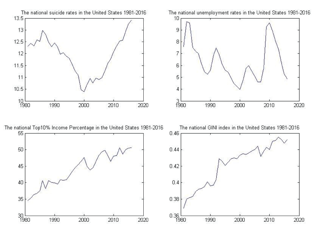
Figure 1: The time trends of the panel data.
The recent study done by Inagaki [23] about the relationship between the suicide rate and income inequality in Japan, found that income inequality and the unemployment rate are positively and significantly related to the suicide rate, and there existed unidirectional Granger-causality from income inequality to the suicide rate in Japan, leading to the conclusion that the fluctuations in Japan’s suicide rate are partially explained by income inequality. Another recent research done by Ayako, Naoki, and so on [24] found that suicide inequalities were substantial in Sweden, and widening suicide inequalities were found with annual increases 3% in men and 10% in women between 1990 and 2007.
Different from theirs, we use state level data in the United States to do the investigation. From table 2, we can find that the Top 10% index has uniform impacts on female, male and overall state suicide rates, while Gini index is not uniformly consistent on the three groups, for it is insignificant on male groups with 1% level and the direction is negative which is hardly to be explained. According to Frank, [18], their new series have modifications and change to the Frank Sommeiller-Price series using data from 2013. For example, California, the table shows that the top 1% income share is 22.7% from the Frank-Sommeiller-Price series, which was constructed using California’s within-state 99th percentile threshold value of $467,882. In the new series, by contrast, they construct the state income share using the US top 1% threshold value from the Piketty-Saez series ($398,318 in 2013). For details, Table 4 was excerpted to see the thresholds that they used to construct the indicators of all states in 2013. With the threshold, California’s share of the US top 1% is 15.7% (i.e., of the 1,679 thousand tax units in the US top 1%, 263 thousand reside in California). For the remaining states, the US top 1% threshold value ($398,318) is applied uniformly for each state within a year. Their Gini series and Top 10% index are constructed based on these series, and the errors could accumulate somehow. But their series are statistically consistent based on their different tests (2014). In other literatures, we find the similar phenomena too, like Jalles & Martin, [25] their Gini index has negative associations within all the groups, based on fixed effects regression and difference GMM estimates.
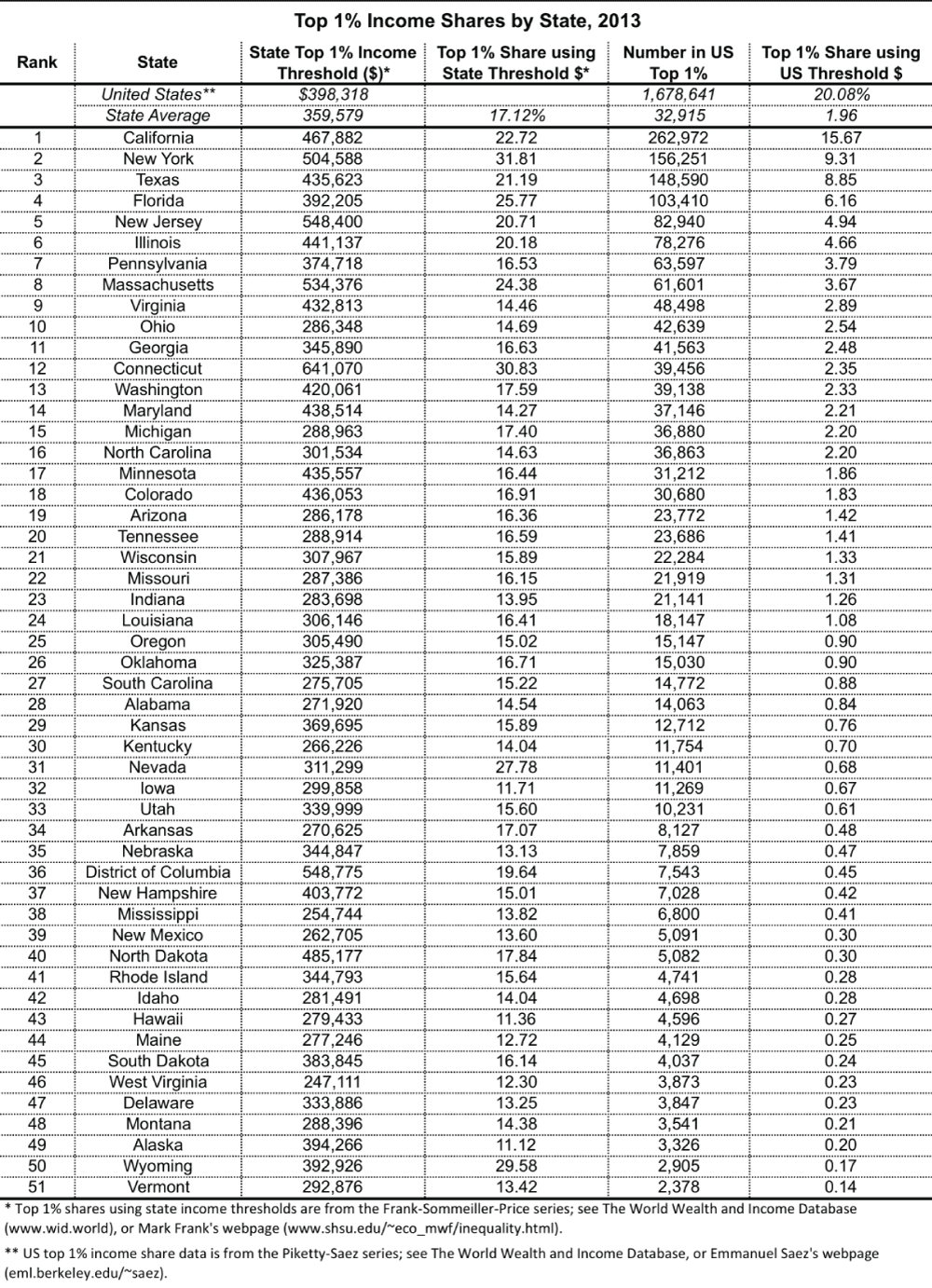
Table 4: Top 1% income thresholds used in each states.
The Wald chi2(3) statistics in all groups (Table 2) are significantly large enough to exclude the null hypothesis. The small p-values from the above tests, which is less than 0.0001, lead to the rejection of the null hypothesis. Finally, the test for autocorrelation of errors presents no evidence of model misspecification.
According to health disparities and inequalities report of the United States from CDC in 2013 and 2016, the socio-economic position may have significant effects on health and mortality including suicides. The reports indicated that racial/ethnic, socioeconomic, and geographic disparities persist in the U.S. adult population, and there are little evidence of improvement since 2009.
This paper aims at giving quantitative verifications of the key points from CDC reports. It is the first to associate the social inequalities with suicides using the state-level dynamic panel data in the United States. The dynamic panel dataset includes the following, the state-level overall, female and male suicide rates, the state-level unemployment rates, the top 10% and GINI index income ratio from 1981 to 2016 in the United States. Arellano-Bond estimate was applied to do the data analyses. The first difference of the regression equation were taken to eliminate the fixed effects. Then, deeper lags of the dependent variable are tested as instruments for the differenced lags of the dependent variable could be endogenous.
It is found that the change of unemployment rates is significant with 1% level and positively impact the changes of the overall suicides rates, female and male suicides rates, the Top10% index has uniform positive impacts on female, male and overall state suicide rates, and Gini index is not uniformly consistent on the three groups. The Gini index has positive association within the overall and female groups, and insignificant and negative association within the male groups.
This paper presents the dynamic panel data analyses with the complete state-level suicide and economic disparities, which is very rare among the historical and recent related researches. In the estimating model, all the coefficients of lagged suicide rates are significant for both 5% level and 1% level. The positive and consistent coefficient estimates of Xi,t-1 confirm that the current year’s measurable increment for suicide rate is adaptive to lagged-one-year’s values.
We also investigated the potential endogeneity problem inferring from the fixed effect estimation illustrated above, and conducted the testing for the auto–regressive error terms with the factor group. The F test statistics shows not only the significance of the alternative models, but also the endogeneity problem. Our results show that there exists large significant error correlations.
Pierce & Schott, [26] investigated the impact of the large economic shock on mortality, and found that exposures to a plausibly exogenous trade liberalization exhibit higher rates of suicide in the different counties. Different from their findings, Autor, Dorn, & Hanson, [27] did not find a statistically significant effect of trade shock on suicide. As they pointed out, on average, trade shocks differentially reduce employment and earnings, and elevate premature mortality among different genders and ages. It would be interesting if we can pursue the related hypothesis in this investigation by including the unemployment rates of different genders and ages as separate controls. However, it is so far very hard to find those panel dataset of different states.
In the future, the work will be extended to including these data, and investigate the associations of the economic and social disparities including education and religions, among groups with different ages and races. The most challenging tasks would be to find the related reliable datasets. Although many datasets have been accessible on the community level, I believe the state-level datasets would be more effective to bring invaluable information to government agencies and community suicide preventions.
- World Health Organization. Mental Health, Suicide data. 2012.
- The U.S. Census Bureau. 2012. https://www.census.gov/topics/income-poverty/wealth.html
- World Data Bank. Datasets of the United States. 2010. https://data.worldbank.org/country/united-states
- Centers for Disease Control and Prevention & National Center for Health Statistics. Suicide Mortality by State. 2016.
- Meyer PA, Yoon PW, Kaufmann RB, Centers for Disease Control and Prevention (CDC). CDC Health Disparities and Inequalities Report — United States. 2013; 62: 3-5. PubMed: https://pubmed.ncbi.nlm.nih.gov/24264483/
- Sun B, Zhang J. Economic and Sociological Correlates of Suicides: Multilevel Analysis of the Time Series Data in the United Kingdom. J Forensic Sci. 2016; 61: 345-351. PubMed: https://pubmed.ncbi.nlm.nih.gov/27404607/
- Antonio A. Income Inequality, Unemployment, and Suicide: A Panel Data Analysis of 15 European Countries. Appl Economics. 2005; 37: 439-451.
- Timothy C, Richard D. The effect of job loss and unemployment duration on suicide risk in the United States: a new look using mass‐layoffs and unemployment duration. Health Econom. 2012; 21: 338-350. PubMed: https://pubmed.ncbi.nlm.nih.gov/21322087/
- Andres AR, Halicioglu F. Determinants of Suicides in Denmark: Evidence from Time Series Data. Health Policy. 2010; 98: 263–269. PubMed: https://pubmed.ncbi.nlm.nih.gov/20667618/
- Phillips J. Factors Associated With Temporal and Spatial Patterns in Suicide Rates Across U.S. States, 1976–2000. Demography. 2013; 50: 591-614. PubMed: https://pubmed.ncbi.nlm.nih.gov/23196429/
- Hintikka J, Saarinen PI, Viinamaki H. Suicide mortality in Finland during an economic cycle, 1985–1995. Scand J Pub Health. 1999; 27: 85–88. PubMed: https://pubmed.ncbi.nlm.nih.gov/10421714/
- Adler NE, Newman K. Socioeconomic Disparities In Health: Pathways And Policies. Health Aff. 2002; 21: 60-76. PubMed: https://pubmed.ncbi.nlm.nih.gov/11900187/
- Adler NE, Rehkopf DH. U.S. disparities in health: descriptions, causes, and mechanisms. Ann Rev Public Health. 2008; 29: 235-252. PubMed: https://pubmed.ncbi.nlm.nih.gov/18031225/
- Ceccherini-Nelli A, Priebe S. Economic Factors and Suicide Rates: Associations over Time in Four Countries. Soc Psychiatry Psychiatr Epidemiol. 2011; 46: 975-982. PubMed: https://pubmed.ncbi.nlm.nih.gov/20652218/
- Yang B, Stack S, Lester D. Suicide and Unemployment: Predicting the Smoothed Trend and Yearly Fluctuations. Soc Eco. 1992; 39-41.
- Stack S. Suicide: A 15-Year Review of the Sociological Literature. Part I: Cultural and Economic Factors. Suicide Life Threat Behav. 2000; 30: 145-162. PubMed: https://pubmed.ncbi.nlm.nih.gov/10888055/
- Swan TT, Sun B, Floss F. Looking at the taxation effect on cross-state smuggling using rational addiction models. J Econo Stud. 2019; 46: 652-670.
- Frank, Mark. W. A New State-Level Panel of Annual Inequality Measures over the Period 1916 – 2005. J Business Strategies. 2014; 31: 241-263.
- National Healthcare Quality and Disparities Report. Rockville, MD: Agency for Healthcare Research and Quality. AHRQ. 2017; 17-0001.
- Manuel A, Stephen B. Some tests of specification for panel data: Monte Carlo evidence and an application to employment equations. Rev Econo Stud. 1991; 58: 277.
- Manual S. Arellano–Bond linear dynamic panel-data. 2014.
- Lin YH, Chen WY. Does unemployment have asymmetric effects on suicide rates? Evidence from the United States: 1928–2013.” Economic Research-Ekonomska Istraživanja. 2018; 31: 1.
- Inagaki K. Income inequality and the suicide rate in Japan: Evidence from cointegration and LA-VAR. J Appl Econo. 2010; 13: P113-133.
- Hiyoshi A, Kondo N, Rostila M. Increasing income-based inequality in suicide mortality among working-age women and men, Sweden, 1990–2007: is there a point of trend change? J Epidemiol Commun Health. 2018; 72: 1009-1015. PubMed: https://pubmed.ncbi.nlm.nih.gov/30021795/
- Jalles JT. Andresen MA. The social and economic determinants of suicide in Canadian provinces. Health Econom Rev. 2015; 5: 1-12. PubMed: https://www.ncbi.nlm.nih.gov/pmc/articles/PMC4314828
- Pierce J, Schott P. Trade Liberalization and Mortality: Evidence from US Counties. Am Econo Rev Insights. 2020; 2: 47-64.
- Autor D, Dorn D, Hanson G. When Work Disappears: Manufacturing Decline and the Falling Marriage-Market Value of Young Men. NBER Working Paper No. 23173. 2017.